The issues an analyst needs to consider when a calibration is
performed are as follows:
- The number of calibration standards – For an initial assessment of the calibration function at least seven different concentrations (including a blank) should be prepared.
A calibration standard is
a solution prepared from a substance or reference material used to calibrate an
instrument.
- The concentration of each of the calibration standards - The standard concentrations should cover, at least, the range of concentrations encountered during the analysis of test samples and be evenly spaced across the range.
- The number of replicates at each concentration - At least duplicate measurements at each concentration level.
- The preparation of the calibration standards - Calibration solutions are prepared from a pure substance with a known purity value or a solution of a substance with a known concentration. The uncertainty associated with the concentration of the standard solution needs to be considered to ensure that it is fir for purpose.
Let’s suppose that we repeat the calibration experiment described in the previous post entitled "What is calibration? Calibrated instruments|Analytical Chemistry" where Instrument Response (Absorbance, A) was determined for a
series of analyte concentrations. This time though the analysis at each
concentration level will be repeated six times and the average absorbance at
each concentration level will be plotted. The average value of a series of
replicate measurements of a physical or chemical quantity is considered to be very close to the true value (or better
approaches the true value as the measurements tend to infinity).
The results obtained are given in Table I.1:
Table I.1: Instrument Response for different analyte A concentrations (analysis was repeated six
times at each concentration level)
Analyte Concentration (μg/l)
|
Instrument Response (Absorbance)
|
Average
Absorbance
|
|||||
0
|
0.0125
|
0.0121
|
0.0122
|
0.0124
|
0.0123
|
0.0123
|
.0123
|
2
|
0.1244
|
0.1240
|
0.1246
|
0.1242
|
0.1248
|
0.1244
|
.1244
|
4
|
0.2500
|
0.2510
|
0.2509
|
0.2507
|
0.2507
|
0.2508
|
.2507
|
6
|
0.3818
|
0.3822
|
0.3820
|
0.3823
|
0.3817
|
0.3820
|
.3820
|
8
|
0.4882
|
0.4886
|
0.4884
|
0.4900
|
0.4878
|
0.4888
|
.4886
|
10
|
0.6400
|
0.6010
|
0.5980
|
0.5993
|
0.5997
|
0.5995
|
.6062
(.5995)1
|
1 The average absorbance when the 0.6400 value is excluded as
outlier.
The questions that we have to answer before plotting the best-fitted
line are as follows:
- Are the experimental data (absorbance values) at each concentration level normally distributed?
- Are there outliers at each concentration level?
- Is the calibration function linear?
The normality of experimental data
can be checked by using the Normal Q-Q Plot.
If all the points are near the straight line (Fig. 1) we have good
evidence for a normal distribution.
Let us select the absorbance values
obtained for the analyte concentration at 10 μg/l (Table I.1).
The Normal Q-Q chart plots the
values you would expect to get if the distribution were normal (expected normal value, Fig. 1a) against the values actually seen
(observed values). The expected values
are a straight diagonal line and the observed values are plotted as individual
points. If the data are normally distributed, then the observed values (blue-red
dots in Fig. 1a) should fall exactly along the straight line. Any deviation of
the dots from the line represents a deviation from normality. Specifically, if
the points are consistently below or above the line or they form an S pattern
then the distribution is not normal.
 |
|
Fig. 1a: A Normal Q-Q Plot
of Instrument Response (Absorbance) of the data given in Table I.1 corresponding to 10 μg/l concentration - Testing if Absorbance values are normally distributed
|
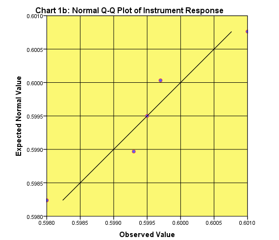
In this case the data are not normally distributed mainly because of the possible outlier point 0.6400 (Table I.1).
If this point will be excluded from the graph we get a Q-Q plot that shows that the distribution of the rest of the data are close to normality (Fig, 1b):
Relevant Posts
Detection of Outliers in Analytical Data - The Grubb's Test
Detection of a Single Outlier| Statistical Analysis
References
1. K. Danzer, L.A. Currie, Pure
& Appl. Chem., Vol. 70, 4, 993-1014 (1998)
2. D. Harvey, “Modern Analytical Chemistry”, McGraw-Hill Companies
Inc., 2000
4.
A. Field, “Discovering
Statistics using SPSS” , Sage Publications Ltd., 2005
5.
V. Barwick, VAM, “Preparation of
Calibration Curves”, LGC Ltd., 2003

No comments:
Post a Comment