Statistical Treatment of Analytical Data - One-Sample t-test in Chemical Analysis
A one-sample t-test is used to compare two means provided that data are normally distributed (plot of the frequencies of data is a histogram of normal distribution). A t-test is a parametric test and relies on distributional assumptions. It is a useful tool in analytical work when two means have to be compared. A situation like this is presented in the following example.
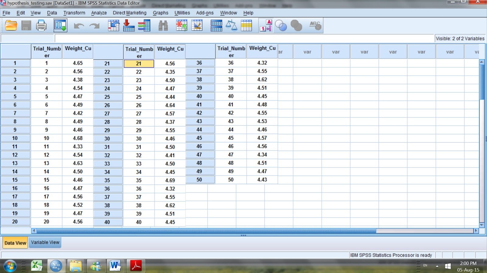
A new analytical instrument is tested in a chemical laboratory by determining the mass m (in mg) of Cu contained in a certain mass (i.e. 1 g) of a certified reference material (CRM). The analysis certificate of the CRM states that the average mass of Cu (in mg) is 4.54 per 1 g of sample. Fifty samples of 1 g of the CRM were analyzed by the new analytical instrument and the results are shown in Fig. I.1. At the 5% level of significance, does the instrument work properly?

A t-test for one sample can be used in this case, a sample mean would be computed and that sample mean would be compared to the specified value given 4.54 mg /g of CRM. A statistical software such as SPSS will be used to do all of the hard work in 5 steps:
Step #1
State the hypotheses:
Ho: The mean mass of Cu in the fifty 1 g samples of CRM analyzed equals 4.54 mg
Ha: The mean mass of Cu in the fifty 1 g samples of CRM analyzed does not equal 4.54 mg
Step #2
Choose a significance level:
In this case is given at the 5% level of significance (or .05)
Step #3
State all the assumptions:
The t-test is a so called parametric test based on the normal distribution. A parametric test is one that requires data from one of the large catalog of distributions that statisticians have studied – such as the normal distribution.
Therefore, the most important assumption in this case is that the results in Fig. I.1 are normally distributed. This can be tested as follows: i) visually by plotting a histogram (Fig. I.2) ii) by using the Kolmogorov-Smirnov test (a nonparametric test).
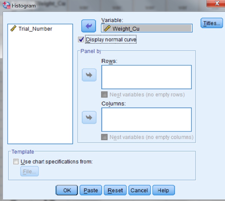
i) In order to conduct visually for normality using SPSS go to Graphs → Legacy Dialogs → Histogram (Fig. I.2) and then choose as variable the one tested in this case Weight_Cu.

Check the box next to Display Normal Curve (Fig. I.3).

The histogram obtained (Fig. I.4) does not appear to have a perfect bell-shaped curve - as a normal distribution curve has - but it is close enough taking into consideration that a sample is tested and not the entire population. There are more data in the middle and less towards the far right or far left. Almost half of the data are below and above the mean 4.50 and there are no any extreme values (outliers). All the above observations show that the assumption of normality seems reasonable and therefore the t-test can be used.

The Kolmogorov-Smirnov test can also be used to evaluate the normality assumption. In order to conduct this test, go to Analyze → Nonparametric Tests → Legacy Dialogs → 1-S K-S (Fig. I.5).

The output shows that the mean mass of Cu in the 50 samples (N=50) is equal to 4.4998 (Mean = 4.4998) with a minimum mass value at 4.32 and a maximum at 4.69 (please notice that the mean mass is close to the mass reported by the CRM certificate). The output also shows that the Asymp. Sig. (2-tailed) is 0.843 (that is also known as the p value) (Fig. I.6). Since the p value is above 0.05 the normality assumption cannot be rejected and therefore the distribution is considered normal.

The p-value expresses the probability that you would be in error if you rejected that the distribution is normal. Therefore, the distribution can be considered normal and the t-test can be used.
To run the t-test using SPSS (version 20) go to Analyze → Compare Means → One-Sample t Test.
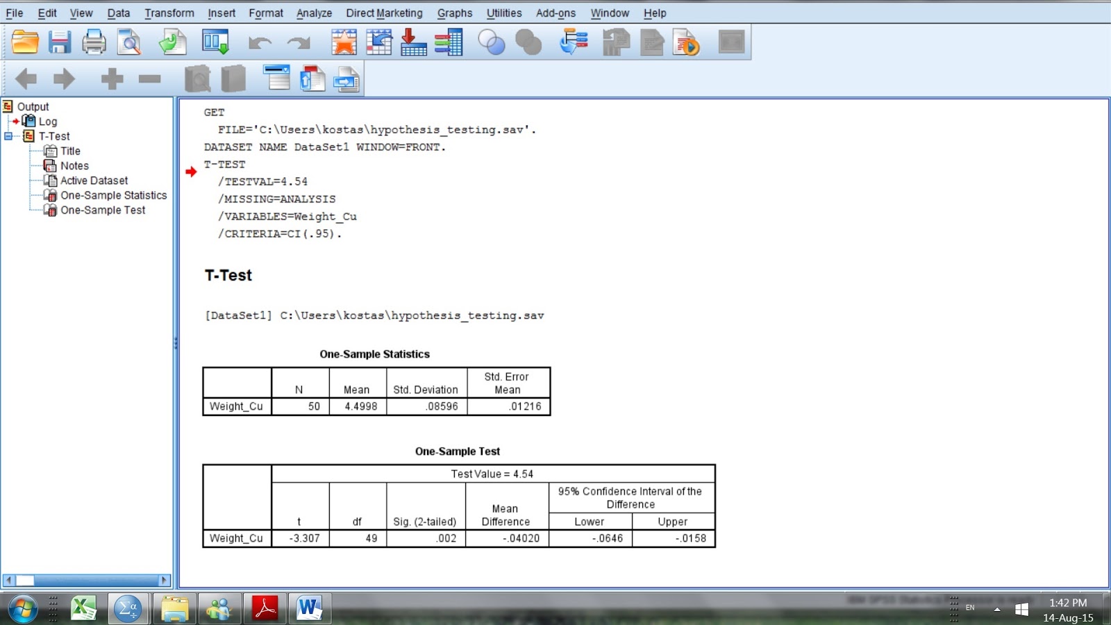
Choose Weight_Cu as the Test Variable and 4.54 (CRM’s mean value) as Test Value (Fig. I.7) and press O.K.

The output shows (Fig. I.8) sample statistics for the test variable Weight_Cu ( N = 50, Mean = 4.4998). The t-test output has a Sig. (2-tailed) p value of 0.002 that is lower than 0.05 and therefore the Null Hypothesis (Ho: The mean mass of Cu in the fifty 1 g samples of CRM analyzed equals 4.54 mg and therefore the instrument works properly) is rejected.

When the null is rejected the alternate hypothesis is considered true (Ha: The mean mass of Cu in the fifty 1 g samples of CRM analyzed does not equal 4.54 mg and therefore the instrument does not work properly).
Relevant Posts
Statistics – Frequency Distributions, Normal Distribution, z-scores
Testing for Normality of Distribution (the Kolmogorov-Smirnov test)
References
- D.B. Hibbert, J.J. Gooding, "Data Analysis for Chemistry", Oxford Univ. Press, 2005
- J.C. Miller and J.N Miller, “Statistics for Analytical Chemistry”, Ellis Horwood Prentice Hall, 2008
- Steven S. Zumdahl, “Chemical Principles” 6th Edition, Houghton Mifflin Company, 2009
- D. Harvey, “Modern Analytical Chemistry”, McGraw-Hill Companies Inc., 2000
- R.D. Brown, “Introduction to Chemical Analysis”, McGraw-Hill Companies Inc, 1982
- S.L.R. Ellison, V.J. Barwick, T.J.D. Farrant, “Practical Statistics for the Analytical Scientist”, 2nd Edition, Royal Society of Chemistry, 2009
- A. Field, “Discovering Statistics using SPSS” , Sage Publications Ltd., 2005
Key Terms
No comments:
Post a Comment