Chemistry Net: Analytical Chemistry - Statistical Analysis of Experimental Data
Showing posts with label Analytical Chemistry - Statistical Analysis of Experimental Data. Show all posts

Comparing several group means by one-way ANOVA - Post Hoc tests using SPSS

Comparing several Group Means by ANOVA using SPSS

Comparing of several Group Means by One-Way ANOVA using SPSS - Post Hoc Tests

In a previous post entitled "Comparing several Group Means by One-Way Anova using SPSS" the one-way ANOVA test was presented. An example was given where the situation encountered was to compare mean results for the concentration of an analyte obtained by threel different methods. The dependent variable was the mean analytical results (labeled Analytical_Result_g) while the independent variable was the method used (labeled Method)

It is common in analytical work to run experiments in which there are three, four or even five levels of the independent variable (that can cause variation of the results in addition to random error of measurements) and in these cases the technique called analysis of variance (ANOVA) is used. ANOVA is an extremely powerful statistical technique for analysis of data that has the advantage that it can be used to analyze situations in which there are several independent variables (or better several levels of the independent variable).

The output of the ANOVA test showed that the mean results of the concentration of the analyte by the three methods used were not equal. In this post we are going to answer which mean differs from which mean by using Post Hoc tests. Post hoc tests (also called post hoc comparisons, multiple comparison tests, follow-up tests) are tests of the statistical significance of differences between group means calculated after - "post"- having done an analysis of variance (ANOVA) that shows an overall difference. The F ratio of the ANOVA indicates that some sort of statistically significant differences exist somewhere among the groups being studied. Post hoc analyses are meant to specify what kind and where.

There are various Post Hoc tests such as: Tukey's Honestly Significant Difference (HSD) test, Scheffe test, Newman-Keuls test and Duncan's Multiple Range test. If the assumption of homogeinity of variance has been met (equal variances assummed) - in our case has been proven in our previous post entitled "Comparing several Group Means by One-Way Anova using SPSS" - Tukey's test is used.

There are many ways to run the exact same ANOVA in SPSS. This time the General Linear Model is going to be used because it will provide us with an estimate for the effect size of our model (labeled as partial eta squared). The effect size will show us what percentage of the variance of the analytical results (of the dependent variable) can be accounted to the different methods used (of the independent variable).

Let us use again the same Example I.1

Example I.1

Figure I.1 shows the analytical results obtained regarding the weight of Au (in grams/ton) in a certified reference material X. Three different methods (Method 1, 2 and 3) were used for the determination and six replicate measurements were made in each case. Is there a significant difference in the means calculated by each method?

Weight of Au (grams/ton) in a certified reference material X determined by 3 different methods - Example ANOVA

In SPSS access the main dialog box using Analyze --------> General Linear Model --------> Univariate (Fig. I.1)

Selecting the General Linear Model, univariate  in SPSS and run the ANOVA test

In SPSS select as Dependent Variable: Analytical_Result_g and as Fixed Factor (independent variable): Method (Fig. I.2). Select also Post Hoc and Options tests.
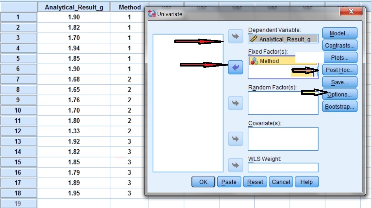
Selecting the Dependent variable (Analytical _Result_g) and the Independent Variable (Method)

The selection Post Hoc is pressed (Fig. I.3) and the independent variable method is selected for the Post Hoc tests (Fig. I.3). Then select the Tukey test and click Continue.

The SPSS dialog box for Post Hoc tests: The  Tukey test is selected

The selection Options is pressed (Fig. I.4) and the Estimates of the effect size is selected. Continue is pressed.

The SPSS dialog box Options: estimates of effect size and homogeinity tests are selected

The SPSS ANOVA output of Between Subjects Effects is shown in Fig. I.5. The mean results for the dependent variable Analytical_Result_g obtained by the 3 different methods differ significantly since the p value denoted by Sig = 0.009 < 0.05. The result for the p value - as expected -is exactly the same with that obtained in the previous post mentionned above. However, an estimate of the effect size is given by this ANOVA test labeled as Partial Eta Squared. The different methods used account for some 47% (given as .470) of the variance in the means of the Analytical_Result_g.

The SPSS Output for Between Subjects Effects with an estimate of the effect size given as partial eta squared

From the results shown in the output of Between Subjects Effects (Fig. I.5) it appears that the 3 means compared differ significantly. But exactly which mean differs from which mean?

Certainly, histograms and the mean table that were given in the post "Comparing several Group Means by One-Way Anova using SPSS" gave us a clue. A more formal answer is given by the Tukey's test in the Multiple Comparisons table (Fig. I.6). Statistically significant mean differences are flagged with an asterisk (*). For instance, the very first line indicates that Method 1 has a mean value 0.2 higher than the mean value of Method 2 and this is statistically significant since Sig = 0.023 < 0.05. Also since the confidence interval is not including zero means that zero difference between these means is unlikely.

The SPSS Output for Post hoc Tests


Method 3 has a mean value 0.02 higher than the mean value of Method 1 and this is not statistically significant since Sig = 0.958 > 0.05. Also since the confidence interval is including zero means that zero difference between these means is likely.


References

  1. D.B. Hibbert, J.J. Gooding, "Data Analysis for Chemistry", Oxford Univ. Press, 2005
  2. J.C. Miller and J.N Miller, “Statistics for Analytical Chemistry”, Ellis Horwood Prentice Hall, 2008
  3. Steven S. Zumdahl, “Chemical Principles” 6th Edition, Houghton Mifflin Company, 2009
  4. D. Harvey, “Modern Analytical Chemistry”, McGraw-Hill Companies Inc., 2000
  5. R.D. Brown, “Introduction to Chemical Analysis”, McGraw-Hill Companies Inc, 1982
  6. S.L.R. Ellison, V.J. Barwick, T.J.D. Farrant, “Practical Statistics for the Analytical Scientist”, 2nd Edition, Royal Society of Chemistry, 2009
  7. A. Field, “Discovering Statistics using SPSS” , Sage Publications Ltd., 2005

Key Terms

comparing several means, analysis of variance,post hoc tests, ANOVA, t-tests,


Statistical Analysis of Experimental Data

Statistical Analysis of Experimental Data - Index

STATISTICAL ANALYSIS OF EXPERIMENTAL DATA


The major objectives of the application of statistics to Science and to chemical analysis are to determine the best value of a series of analytical results obtained with a particular sample and to give some indication of the reliability of the analysis.

As scientists, we are interested in finding results that apply to an entire population of people/ or material/ or chemical substance.

There is no doubt that it would be extremely expensive and impractical to analyze the entire population to draw conclusions about certain variables.
Therefore, in most cases we collect data from a small subset of the population (known as sample) and use these data to infer things about the population as a whole. This small sample’s  statistical measurements is the “model” for the entire population.


References

  1. D. Harvey,  “Modern Analytical Chemistry”, McGraw-Hill Companies Inc., (2000)
  2. L.R. Ellison, V.J. Barwick, T.J.D. Farrant, “Practical Statistics for the Analytical Scientist”, 2nd Edition, Royal Society of Chemistry, (2009) 
  3. D.B. Hibbert, J.J. Gooding, "Data Analysis for Chemistry", Oxford Univ. Press, (2005)
  4. J.C. Miller, J.N. Miller, "Statistics for Analytical Chemistry",3 Sub edition, Ellis Horwood Ltd, (1993)

Comparing several Group Means by ANOVA using SPSS

Comparing several Group Means by ANOVA using SPSS

Comparing of several Group Means by One-Way ANOVA using SPSS

In a previous post entitled "One-Sample T-Test in Chemical Analysis – Statistical Treatment of Analytical Data" the statistical tests presented were limited to situations in which there were only up to two levels of the independent variable (i.e. up to two experimental groups, two experimental conditions) and the data were normally distributed (histogram of normal distribution was obtained by plotting data). Methods were described for comparing two means to test whether they differ significantly. However, in analytical work there are often more than two means to be compared. Some situations encountered are:

  • comparing the mean results for the concentration of an analyte by several different methods
  • comparing the mean results obtained for the analysis of a sample by several different laboratories
  • comparing the mean concentration of a solute A in solution for samples stored under different conditions
  • comparing the mean results for the determination of an analyte from portions of a sample obtained at random (checking the purity of a sample)

Therefore, it is common in analytical work to run experiments in which there are three, four or even five levels of the independent variable (that can cause variation of the results in addition to random error of measurements) and in these cases the tests described in previous posts are inappropriate. Instead a technique called analysis of variance (ANOVA) is used. ANOVA is an extremely powerful statistical technique for analysis of data that has the advantage that it can be used to analyze situations in which there are several independent variables (or better several levels of the independent variable). In the examples given above levels of the independent variable are the different methods used, the different laboratories, the different conditions under which the solutions were stored.

The so called one-way ANOVA is presented in this post since there is one factor in addition to the random error of the measurements that causes variation of the results (methods, laboratories, storage conditions respectively). More complex situations in which there are two or more factors (i.e methods and laboratories, methods and storage conditions), possibly interacting with each other are going to be presented in another post.

When the one-way ANOVA test should be used?

One-way ANOVA should be used when there is only one factor being considered and replicate data from changing the level of that factor are available. One-way ANOVA will answer the question: Is there a significant difference between the mean values (or levels), given that the means are calculated from a number of replicate measurements? It tests the hypothesis that all group means are equal. An ANOVA produces an F-statistic or F-ratio, which is similar to a t-test (t-statistic) in that it compares the amount of systematic variance in the data to the amount of unsystematic variance.

Why not use several t-tests instead of ANOVA?

Imagine a situation in which there were three experimental conditions (Method 1, Method 2 and Method 3) and we were interested in comparing differences in the means of the results of these three methods. If we were to carry out t-tests on every pair of methods, then we would have to carry out three separate tests: one to compare means of Method 1 and 2, one to compare means of Method 1 and 3 and one of Method 2 and 3. Not only is this a lot of work but the chance of reaching a wrong conclusion increases. The correct way to analyse this sort of data is to use one-way ANOVA.

Results from statistical analysis have a certain value only if all relevant assumptions are met. For a one-way ANOVA these are:

  1. Normality: The dependent variable is normally distributed within each population (ANOVA is a parametric test based on the normal distribution). Since most of the time we do not have a large amount of data it is difficult to prove any departure from normality. It has been shown, however, that even quite large deviations from normality do not affect the ANOVA test. ANOVA is a robust method with respect to violations of normality. If there is a large amount of data tests for normality can be used such as the Normal Q-Q plots, the Shapiro-Wilk test of normality, plotting histograms and skewness and kurtosis.
  2. Homoscedasticity: The variance (spread) between groups (populations) is homogeneous (all populations have the same variance). If this is not the case (this happens often in chemical analysis) then the F-test can suggest a statistically significant difference where none is present. The best way to check for this is to plot the data. There are also a number of tests for heteroscedasity like Bartlett's test and Levene's test. Homoscedasticity not holding is less serious when the sample sizes are equal. It may be also overcome this type of problem in the data by transforming it by taking for example logarithms (logs)
  3. Independent data: This often holds if each case (row of cells) represents a unique observation

If assumptions 1 and 2 seem seriously violated then the Kruskal-Wallis test can be used instead of ANOVA. This test is a non-parametric test and therefore does not require normally distributed data.

The principle of the one-way ANOVA test is more easily understood by means of the following example.

Example I.1

Figure I.1 shows the analytical results obtained regarding the weight of Au (in grams/ton) in a certified reference material X. Three different methods (Method 1, 2 and 3) were used for the determination and six replicate measurements were made in each case. Is there a significant difference in the means calculated by each method?

Weight of Au (grams/ton) in a certified reference material X determined by 3 different methods - Example ANOVA

Before running an ANOVA test let us first plot our data using a histogram (frequency distribution curve). The results in Fig. I.1 have been inserted in an SPSS spreadsheet. In SPSS access the main dialog box using Graphs --------> Legacy Dialogs --------> Histogram

The following histogram is obtained (Fig. I.2). A split histogram gives information regarding the three assumptions mentioned above.

Histograms of the frequencies of the results of the variable Analytical_Result_g vs. values of the dependent variable Analytical_Result_g for the three methods used

  1. Normality: All distributions look reasonably normal even though there is not a large amount of data. The dependent variable seems normally distributed within each population. It has been shown, however, that even quite large deviations from normality do not affect the ANOVA test.
  2. Homoscedasticity: The two histograms - first and third - are roughly equally wide. The second seems to be wider due to a outlier. It seems as though the results have roughly equal variances over the three methods. As a rule of thumb variances are unequal when the larger variance is more than 4 times the smaller variance. This is not the case in this example. Levene's test is going to be used to prove that variances for the three methods are equal in a formal way.
  3. Independent data: Data are independent since each case (row of cells) represents a unique observation

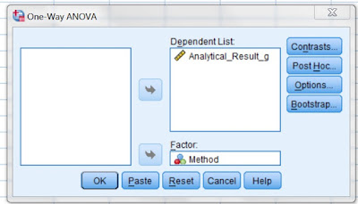
In SPSS access the main dialog box using Analyze --------> Compare Means --------> One-Way Anova (Fig. I.3) and select as Dependent List (variable): Analytical_Result_g and as Factor: Method. Press O.K. (Fig. I.4). The means of the analytical results obtained by Method 1, 2 and 3 (methods are a factor that may affect the means) are compared. The question that has to be answered is if the differences between these means are statistically significant or these mean values are the same.

One-way ANOVA using SPSS - Selecting Analyze, Compare Means, One-Way Anova

One-way ANOVA using SPSS - Selecting the Dependent Variable: Analytical_Result_g and the factor that may affect the means (the three methods Method 1,2,3)

The selection Options is pressed (Fig. I.4) and Descriptive Statistics, Homogeneity of Variance Test and Means Plot is checked in the one-way ANOVA SPSS dialog box and Continue is pressed (Fig. I.5).

The SPSS dialog box One-Way Anova: Options

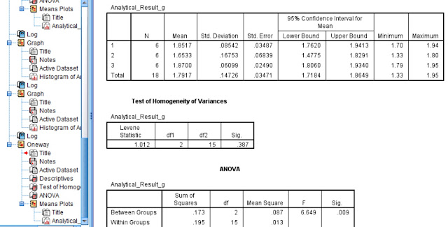
After running the ANOVA test the following results are obtained (Fig. I.6):

  1. A Descriptives table for the dependent variable Analytical_Result_g. Where N is the number of replicates by each method (N=6). The mean weights of Au are almost equal when Methods 1 and 3 were used - 1.85 and 1.87 respectively - and they differ from the mean of Method 2 which is 1.65. Our main research question is whether these means differ significantly for the three different methods.
  2. A table for the test of Homogeneity of Variances (Levene's test). It checks whether the variances of the results obtained by the three methods differ significantly. If p ‹ 0.05 then they differ significantly. In this case p = 0.387 › 0.05 and therefore the variances of the three means do not differ significantly. Therefore, the ANOVA test was the right choice.
  3. An ANOVA table. Where the degrees of freedom df for Between Groups and Within Groups are given (2 and 15 respectively) and the F statistic F= 6.649. The p value denoted by Sig = 0.009 ‹ 0.05 indicates that the three means differ significantly due to the different analytical methods.

The SPSS One-Way Anova Output with a Descriptives, Test of Homogeinity of variances and ANOVA table


References

  1. D.B. Hibbert, J.J. Gooding, "Data Analysis for Chemistry", Oxford Univ. Press, 2005
  2. J.C. Miller and J.N Miller, “Statistics for Analytical Chemistry”, Ellis Horwood Prentice Hall, 2008
  3. Steven S. Zumdahl, “Chemical Principles” 6th Edition, Houghton Mifflin Company, 2009
  4. D. Harvey, “Modern Analytical Chemistry”, McGraw-Hill Companies Inc., 2000
  5. R.D. Brown, “Introduction to Chemical Analysis”, McGraw-Hill Companies Inc, 1982
  6. S.L.R. Ellison, V.J. Barwick, T.J.D. Farrant, “Practical Statistics for the Analytical Scientist”, 2nd Edition, Royal Society of Chemistry, 2009
  7. A. Field, “Discovering Statistics using SPSS” , Sage Publications Ltd., 2005

Key Terms

comparing several means, analysis of variance, ANOVA, t-tests,


Testing for Normality of Distribution (the Kolmogorov-Smirnov test)

Testing for Normality of Distribution (the Kolmogorov-Smirnov test)

Testing for Normality of Distribution (Kolmogorov-Smirnov test) using the Online Normal Distribution Calculator

Many statistical tests (t-test, f-test, one-way ANalysis Of VAriance ANOVA) assume that data used are drawn from a normal population. Although the chi-squared test can be used to test this assumption it should be used only if there are 50 or more data points, so it is of limited value in analytical work, when we often have only a small set of data. There Kolmogorov-Smirnov test (a nonparametric test).

The Kolmogorov-Smirnov test – included in SPSS - has been used in a previous post entitled "Statistical Treatment of Analytical Data - One-Sample t-test in Chemical Analysis" for testing that data is normally distributed.

The principle of the method involves comparing the sample cumulative distribution function with the cumulative distribution function of the hypothesized distribution. If the experimental data depart substantially from the expected distribution, the two functions will be widely separated. If, however, the data are closely in accord with the expected distribution, the two functions will never be very far apart. The test statistic is given by the maximum difference between the two functions (Dx)exp and is compared in the usual way with a set of tabulated values (D)crit.

When the Kolmogorov–Smirnov method is used to test whether a distribution is normal, the original data are transformed into the standard normal variable, z.

This is done by using the equation:

z = (x – μ) / s

where μ is the mean and s the standard deviation of the data.

The data are next transformed by using the above equation and then the Kolmogorov–Smirnov method is applied. This test is illustrated in the example given in “Statistical Treatment of Analytical Data - One-Sample t-test in Chemical Analysis” using SPSS. The Kolmogorov–Smirnov test in SPSS shows that the data tested are normally distributed at the 95% confidence level (Figure I.1)

Fig. I.1: Screenshot of the Kolmogorov-Smirnov test in SPSS (95% confidence level) for the data given in the post entitled “Statistical Treatment of Analytical Data - One-Sample t-test in Chemical Analysis”

The same data are tested below using an online Normal Distribution Calculator (Kolmogorov-Smirnov test).

The data are inserted or copied in the yellow-labeled cells and the confidence level is selected from the drop-down list (in this case 95%). The median, 15% trimmed mean, mean, standard deviation, # of data, Dexp, Dcrit and the Result is calculated (Fig. I.2).

Fig. I.2: Screenshot of the output of the Kolmogorov-Smirnov test given by the online Normal Distribution Calculator (95%confidence level) for the data given in the post entitled “One-Sample T-Test in Chemical Analysis – Statistical Treatment of Analytical Data ”

The result is consistent with the SPSS test showing that the tested data are normally distributed. A first indication of normally distributed data is given by the fact that mean≈ median ≈ 15% trimmed mean.

The Online Normal Distribution Calculator is given below:


References

  1. D.B. Hibbert, J.J. Gooding, "Data Analysis for Chemistry", Oxford Univ. Press, 2005
  2. J.C. Miller and J.N Miller, “Statistics for Analytical Chemistry”, Ellis Horwood Prentice Hall, 2008
  3. Steven S. Zumdahl, “Chemical Principles” 6th Edition, Houghton Mifflin Company, 2009
  4. D. Harvey, “Modern Analytical Chemistry”, McGraw-Hill Companies Inc., 2000
  5. R.D. Brown, “Introduction to Chemical Analysis”, McGraw-Hill Companies Inc, 1982
  6. S.L.R. Ellison, V.J. Barwick, T.J.D. Farrant, “Practical Statistics for the Analytical Scientist”, 2nd Edition, Royal Society of Chemistry, 2009
  7. A. Field, “Discovering Statistics using SPSS” , Sage Publications Ltd., 2005

Key Terms

statistical tests, normal population, chi-squared test, data points, plotting a histogram, QQ plot, Kolmogorov-Smirnov test

Dixon's Q-test Calculator - Detection of a single outlier

Dixon' Q test calculator

Dixon's Q-test Calculator - Detection of a single outlier


Dixon’s test (or the Q-test) has been described in a previous post entitled “Detection of a Single Outlier|Statistical Analysis|Quantitative Data ”. The test is popular because the calculations involved are simple. A solved example is given in the above post.

Are there any limitations to Dixon’s Q-test?

  • The data excluding  the possible outlier must be normally distributed (use the Kolmogorov-Smirnov test to check if data is normally distributed)
  • The Q-test is valid for the detection of a single outlier (it cannot be used for a second time on the same set of data). Other forms of Dixon’s Q-test can be applied to the detection of multiple outliers.
  • The Q-test should be applied with caution – the same applies to all statistical tests used for rejecting data - since there is a probability, equal to the significance level a (a =0.05 at the 95% confidence level) that an outlier identified by the Q-test actually is not an outlier.

Moreover, if two suspect values occur, both of them might be at high end of the measurement range, both at the low end, or one at the high end and one at the low end. In situations like these the test may give erroneous results. As an example consider the following data tested for outliers:

4.0, 4.1, 4.2, 4.3, 4.3, 4.9, 5.1

Two of the above values (4.9 and 5.1) are suspiciously high compared with the mean of the data, yet if Q were calculated (at the 95% confidence level) would give that the tested value 5.1 is not an outlier at the 95% confidence level. Clearly, the possible outlier 5.1 has been masked by the other possible outlier 4.9 giving a low value for Q compared to Qcrit.

An online calculator is given below that can identify outliers in a data set at  six different confidence levels (80%, 90%, 95%, 96%, 98%, 99%). To test a data set for possible outliers follow the steps below:

  • Check that data is normally distributed (Kolmogorov-Smirnov test, Q-Q plot)
  • Type data in the yellow-labeled cells
  • Select the confidence level from the drop-down list
  • See the tested value and the results


Relevant Posts

Detection of a Single Outlier|Statistical Analysis|Quantitative Data

Detection of Outliers in Analytical Data – The Grubb’s Test

Calibration and Outliers - Statistical Analysis


References

  1. D. B. Rorabacher,  Anal. Chem., 63, 139–146, (1991)
  2. D. Harvey,  “Modern Analytical Chemistry”, McGraw-Hill Companies Inc., 2000
  3. R.D. Brown, “Introduction to Chemical Analysis”, McGraw-Hill Companies Inc., 1982
  4. J. N. Miller, J. C. Miller, "Statistics and Chemometrics for Analytical Chemistry", 6th Edition, Pearson, 2010

Key Terms

Dixon's q test calculator, calculator online, detecting outlier online, normal distribution, detection of a single outlier